Potential evapotranspiration under warming and elevated \(CO_2\) concentration

M. Vremec, R.A. Collenteur University of Graz, 2021

In this notebook it is shown how to estimate Potential Evapotranspiration under elevated \(CO_2\) conditions and an increase in temperature. The work follows the suggestions made by Yang et al. (2019) to include the sensitivity of stomatal resistance to \(CO_2\) in the Penman-Monteith equation.

Yang, Y., Roderick, M.L., Zhang, S. et al. Hydrologic implications of vegetation response to elevated CO2 in climate projections. Nature Clim Change 9, 44–48 (2019). https://doi.org/10.1038/s41558-018-0361-0

import pandas as pd
import numpy as np
import matplotlib.pyplot as plt

import pyet as pyet

1. Load daily data from ZAMG (Messstationen Tagesdaten)

station: Graz Universität 16412

Selected variables:

• globalstrahlung (global radiation), J/cm2 needs to be in MJ/m3d, ZAMG abbreviation - strahl

• arithmetische windgeschwindigkeit (wind speed), m/s, ZAMG abbreviation - vv

• relative feuchte (relative humidity), %, ZAMG abbreviation - rel

• lufttemparatur (air temperature) in 2 m, C, ZAMG abbreviation - t

• lufttemperatur (air temperature) max in 2 m, C, ZAMG abbreviation - tmax

• lufttemperatur (air temperature) min in 2 m, C, ZAMG abbreviation - tmin

• latitute and elevation of a station

#read data
data_16412 = pd.read_csv('data/example_1/klima_daily.csv', index_col=1, parse_dates=True)
data_16412

	station	strahl	rel	t	tmax	tmin	vv
time
2000-01-01	16412	300.0	80.0	-2.7	0.5	-5.8	1.0
2000-01-02	16412	250.0	86.0	0.2	2.5	-2.1	1.0
2000-01-03	16412	598.0	86.0	0.6	3.6	-2.4	1.0
2000-01-04	16412	619.0	83.0	-0.5	4.5	-5.5	1.0
2000-01-05	16412	463.0	84.0	-0.1	5.4	-5.5	1.0
...	...	...	...	...	...	...	...
2021-11-07	16412	852.0	74.0	8.5	12.2	4.7	1.6
2021-11-08	16412	553.0	78.0	7.5	10.4	4.5	1.6
2021-11-09	16412	902.0	67.0	7.1	11.7	2.4	2.7
2021-11-10	16412	785.0	79.0	5.3	10.1	0.4	2.1
2021-11-11	16412	194.0	91.0	5.1	6.5	3.7	1.1

7986 rows × 7 columns

# Convert Glabalstrahlung J/cm2 to MJ/m2 by dividing to 100

meteo = pd.DataFrame({"time":data_16412.index, "tmean":data_16412.t, "tmax":data_16412.tmax, "tmin":data_16412.tmin, "rh":data_16412.rel, 
                      "wind":data_16412.vv, "rs":data_16412.strahl/100})
time, tmean, tmax, tmin, rh, wind, rs = [meteo[col] for col in meteo.columns]

lat = 47.077778 * np.pi / 180  # Latitude of the meteorological station, converting from degrees to radians
elevation = 367  # meters above sea-level

2.Estimate potential evapotranspiration under RCP scenarios

# the first element in the list includes the rise in temperature, and the CO2 concentration
rcp_26 = [1.3, 450]
rcp_45 = [2, 650]
rcp_85 = [4.5, 850]

def pe_cc(tincrease, co2):
    pe = pyet.pm(tmean+tincrease, wind, rs=rs, elevation=elevation, lat=lat, 
                 tmax=tmax+tincrease, tmin=tmin+tincrease, rh=rh, co2=co2)
    return pe

# Estimate evapotranspiration with four different methods and create a dataframe
pet_df = pd.DataFrame()
pet_df["amb."] = pe_cc(0, 420)
pet_df["RCP 2.6"] = pe_cc(rcp_26[0], rcp_26[1])
pet_df["RCP 4.5"] = pe_cc(rcp_45[0], rcp_45[1])
pet_df["RCP 8.5"] = pe_cc(rcp_85[0], rcp_85[1])

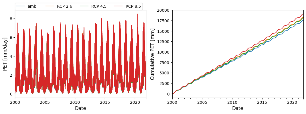
fig, axs = plt.subplots(figsize=(13,4), ncols=2)
pet_df.plot(ax=axs[0])
pet_df.cumsum().plot(ax=axs[1], legend=False)

axs[0].set_ylabel("PET [mm/day]", fontsize=12)
axs[1].set_ylabel("Cumulative PET [mm]", fontsize=12)
axs[0].legend(ncol=6, loc=[0,1.])
for i in (0,1):
    axs[i].set_xlabel("Date", fontsize=12)