Potential Evapotranspiration from CoAgMET data

M. Vremec, University of Graz, 2021

In this notebook it is shown how to compute (reference) evapotranspiration (\(ET_0\)) from meteorological data observed by the Colorado State University (CoAgMET) at Holyoke in Colorado, USA. The notebook also includes a comparison between \(ET_0\) estimated using pyet (FAO56) and \(ET_0\) available from CoAgMET. According to CoAgMET documentation, the provided reference evapotranspiration is estimated using ASCE reference evapotranspiration for short reference grass (Wright, 2000), which corresponds to the FAO-56 method used with pyet.

Source: https://coagmet.colostate.edu/station/selector

import numpy as np
import pandas as pd
import matplotlib.pyplot as plt

import pyet as pyet
pyet.show_versions()

Python version: 3.11.6 (main, Feb  1 2024, 16:47:41) [GCC 11.4.0]
Numpy version: 1.26.4
Pandas version: 2.2.1
xarray version: 2024.2.0
Pyet version: 1.3.2

1. Load CoAgMET Data

data = pd.read_csv("data/example_4/et_coagmet.txt", parse_dates=True, index_col="date")
data

	name	tavg	tmax	tmin	rhmax	rhmin	solar	windrun	et_asce	et_pk	et_asce0
date
2020-01-01	hyk02	-0.8	9.4	-8.9	0.929	0.470	63.1	203.1	1.9	1.9	1.2
2020-01-02	hyk02	0.8	7.2	-4.2	0.902	0.568	107.4	314.7	1.7	1.7	1.1
2020-01-03	hyk02	-0.4	5.0	-4.7	0.855	0.448	76.2	239.6	1.7	1.3	1.1
2020-01-04	hyk02	4.1	16.1	-4.8	0.893	0.224	97.6	253.7	4.0	1.7	2.4
2020-01-05	hyk02	0.5	8.2	-6.9	0.820	0.232	102.3	312.2	3.1	1.9	1.9
...	...	...	...	...	...	...	...	...	...	...	...
2020-12-27	hyk02	2.2	8.9	-6.2	0.967	0.318	98.6	324.5	2.8	1.6	1.7
2020-12-28	hyk02	-4.0	0.0	-10.1	0.994	0.878	26.2	248.3	0.4	0.6	0.3
2020-12-29	hyk02	-4.7	-1.1	-10.8	0.983	0.737	55.6	441.7	0.8	0.6	0.5
2020-12-30	hyk02	-8.4	2.2	-14.6	0.939	0.489	111.5	197.9	1.2	1.0	0.8
2020-12-31	hyk02	-6.3	3.4	-15.3	0.929	0.459	109.0	99.9	0.9	0.6	0.6

366 rows × 11 columns

et0_coagmet = data["et_asce0"]

meteo = pd.DataFrame({"tmean":data["tavg"], 
                      "tmax":data["tmax"],
                      "tmin":data["tmin"], 
                      "rhmax":data["rhmax"]*100,
                      "rhmin":data["rhmin"]*100, 
                      "u2":data["windrun"]*1000/86400,
                      "rs":data["solar"]*86400/1000000})

tmean, tmax, tmin, rhmax, rhmin, wind, rs = [meteo[col] for col in meteo.columns]
lat = 40.49 * np.pi / 180

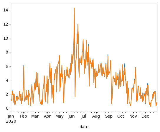
2. Comparison: pyet FAO56 vs CoAgMET ASCE

et0_fao56 = pyet.pm_fao56(tmean, wind, rs=rs, elevation=1138, lat=lat, 
                         tmax=tmax, tmin=tmin, rhmax=rhmax, rhmin=rhmin)

et0_fao56.plot()
et0_coagmet.plot();

3. Plot the results

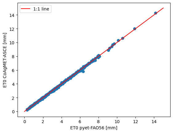
We now plot the evaporation time series against each other to see how these compare.

plt.scatter(et0_fao56, et0_coagmet)
plt.plot([0,15],[0,15], color="red", label="1:1 line")
plt.legend()
plt.xlabel("ET0 pyet-FAO56 [mm]")
plt.ylabel("ET0 CoAgMET-ASCE [mm]");