Potential Evapotranspiration from KNMI data#
R.A. Collenteur, Eawag, 2023
Data source: KNMI - https://dataplatform.knmi.nl/
In this notebook it is shown how to compute (potential) evapotranspiration from meteorological data using PyEt. Meteorological data is observed by the KNMI at De Bilt in the Netherlands.
import pandas as pd
import matplotlib.pyplot as plt

import pyet
pyet.show_versions()
Python version: 3.11.14 (main, Apr 27 2026, 17:28:30) [GCC 11.4.0]
Numpy version: 2.4.4
Pandas version: 2.3.3
xarray version: 2026.4.0
Pyet version: 1.5.0
1. Load KNMI Data#
We first load the raw meteorological data observed by the KNMI at De Bilt in the Netherlands. This datafile contains a lot of different variables, please see the end of the notebook for an explanation of all the variables.
data = pd.read_csv("data/example_3/etmgeg_260.txt", skiprows=46, delimiter=",",
                   skipinitialspace=True, index_col="YYYYMMDD", parse_dates=True).loc["2018",:]
data.head()
| # STN | DDVEC | FHVEC | FG | FHX | FHXH | FHN | FHNH | FXX | FXXH | ... | VVNH | VVX | VVXH | NG | UG | UX | UXH | UN | UNH | EV24 | |
|---|---|---|---|---|---|---|---|---|---|---|---|---|---|---|---|---|---|---|---|---|---|
| YYYYMMDD | |||||||||||||||||||||
| 2018-01-01 | 260 | 225 | 45 | 50 | 90 | 2 | 10 | 18 | 190.0 | 2.0 | ... | 2.0 | 75.0 | 3.0 | 7.0 | 84 | 96 | 17 | 73 | 1 | 3 |
| 2018-01-02 | 260 | 216 | 39 | 45 | 80 | 24 | 20 | 1 | 140.0 | 24.0 | ... | 19.0 | 75.0 | 8.0 | 7.0 | 88 | 96 | 3 | 80 | 8 | 2 |
| 2018-01-03 | 260 | 257 | 82 | 88 | 120 | 11 | 70 | 4 | 290.0 | 3.0 | ... | 1.0 | 75.0 | 4.0 | 8.0 | 73 | 95 | 1 | 65 | 9 | 1 |
| 2018-01-04 | 260 | 238 | 51 | 56 | 90 | 20 | 30 | 14 | 180.0 | 20.0 | ... | 14.0 | 80.0 | 21.0 | 8.0 | 82 | 97 | 14 | 67 | 21 | 2 |
| 2018-01-05 | 260 | 225 | 38 | 40 | 60 | 1 | 20 | 17 | 150.0 | 16.0 | ... | 15.0 | 75.0 | 1.0 | 6.0 | 87 | 96 | 17 | 71 | 3 | 2 |
5 rows × 40 columns
2. Estimating potential evapotranspiration#
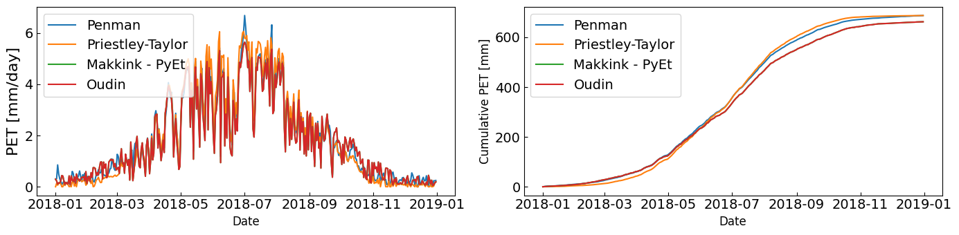
Now that we have the input data, we can estimate potential evapotranspiration with different estimation methods. Here we choose the Penman, Priestley-Taylor, Makkink, and Oudin methods.
# Preprocess the input data
meteo = pd.DataFrame({"tmean":data.TG/10, "tmax":data.TX/10, "tmin":data.TN/10,
                      "rh":data.UG, "wind":data.FG/10, "rs":data.Q/100})
tmean, tmax, tmin, rh, wind, rs = [meteo[col] for col in meteo.columns]
pressure =  data.PG / 100  # to kPa
wind = data.FG / 10  # to m/s
lat = 0.91  # Latitude of the meteorological station
elevation = 4  # meters above sea-level

# Estimate evapotranspiration with four different methods
pet_penman = pyet.penman(tmean, wind, rs=rs, elevation=4, lat=0.91, tmax=tmax, tmin=tmin, rh=rh)
pet_pt = pyet.priestley_taylor(tmean, rs=rs, elevation=4, lat=0.91, tmax=tmax, tmin=tmin, rh=rh)
pet_makkink = pyet.makkink(tmean, rs, elevation=4, pressure=pressure)
pet_oudin = pyet.oudin(tmean, lat=0.91)
3. Plot the results#
We plot the cumulative sums to compare the different estimation methods.
fig, axs = plt.subplots(figsize=(14,3.5), ncols=2)

pet = [pet_penman, pet_pt, pet_makkink, pet_makkink]
names = ["Penman", "Priestley-Taylor", "Makkink - PyEt", "Oudin"]

for df, name in zip(pet, names):
    axs[0].plot(df,label=name)
    axs[1].plot(df.cumsum(),label=name)

axs[0].set_ylabel("PET [mm/day]", fontsize=16)
axs[1].set_ylabel("Cumulative PET [mm]", fontsize=12)

for i in (0,1):
    axs[i].set_xlabel("Date", fontsize=12)
    axs[i].legend(loc=2, fontsize=14)
    axs[i].tick_params("both", direction="in", labelsize=14)
plt.tight_layout()

#plt.savefig("Figure1.png", dpi=300)
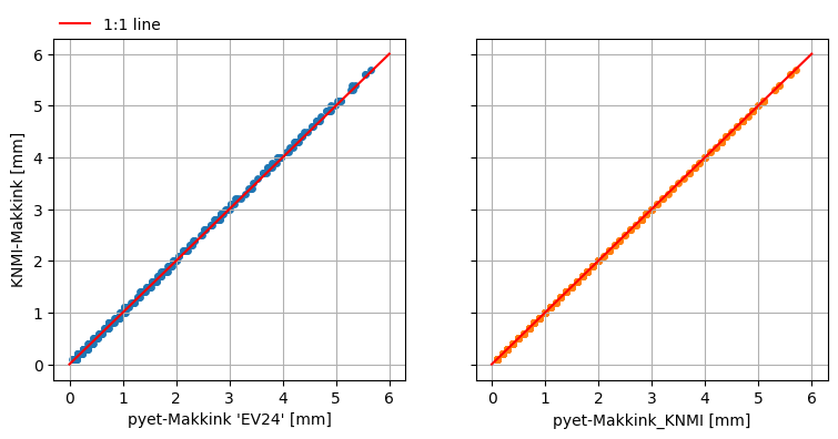
4. Comparison: pyet Makkink vs KNMI Makkink#
The KNMI also provides Makkink potential evapotranspiration data (column EV24). We can now compare the results from Pyet and the KNMI to confirm that these are roughly the same. Pyet also has a method makkink_knmi that calculates exactly the same Makkink evaporation as the KNMI but that is only suitable for the Netherlands.
pet_knmi = data.EV24 / 10  # Makkink potential evaporation computen by the KNMI for comparison
pet_makkink_knmi = pyet.makkink_knmi(tmean, rs).round(1) # same as pet_knmi (if rounded up to 1 decimal) but calculated from tmean and rs

# Plot the two series against each other
_, ax = plt.subplots(1, 2, figsize=(9,4), sharex=True, sharey=True)
ax[0].scatter(pet_makkink, pet_knmi, s=15, color="C0")
ax[0].plot([0,6],[0,6], color="red", label="1:1 line")
ax[0].set_xlabel("pyet-Makkink 'EV24' [mm]")
ax[0].grid()

ax[1].scatter(pet_makkink_knmi, pet_knmi, s=15, color="C1")
ax[1].plot([0,6],[0,6], color="red")
ax[1].set_xlabel("pyet-Makkink_KNMI [mm]")
ax[1].grid()

ax[0].set_ylabel("KNMI-Makkink [mm]")
ax[0].legend(loc=(0,1), frameon=False)
<matplotlib.legend.Legend at 0x7410d7514a90>
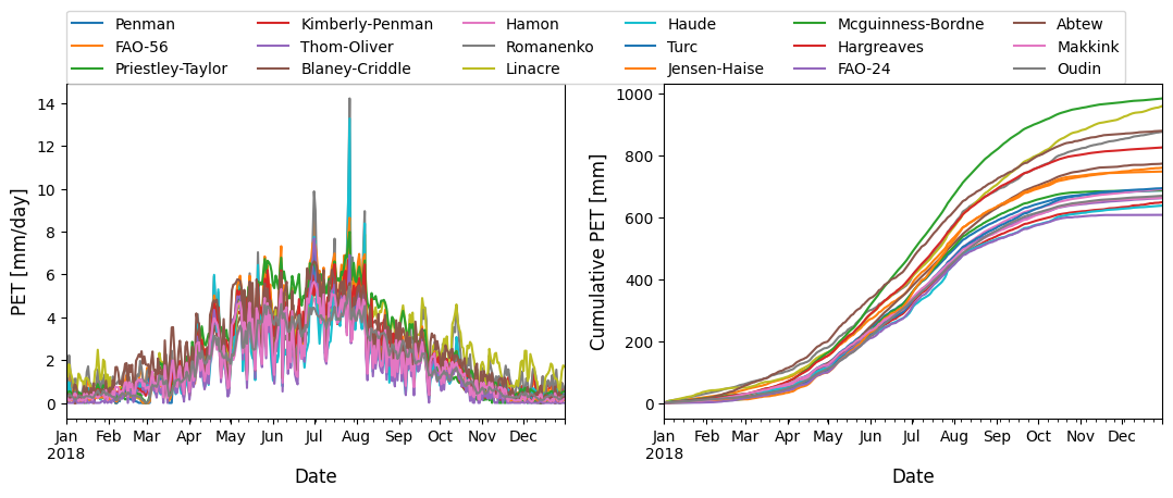
5. Estimation of PET - all methods#
pet_df = pyet.calculate_all(tmean, wind, rs, elevation, lat, tmax=tmax,
                                tmin=tmin, rh=rh)
fig, axs = plt.subplots(figsize=(13,4), ncols=2)
pet_df.plot(ax=axs[0])
pet_df.cumsum().plot(ax=axs[1], legend=False)

axs[0].set_ylabel("PET [mm/day]", fontsize=12)
axs[1].set_ylabel("Cumulative PET [mm]", fontsize=12)
axs[0].legend(ncol=6, loc=[0,1.])
for i in (0,1):
    axs[i].set_xlabel("Date", fontsize=12)
#plt.savefig("PET_methods.png", dpi=300)
References#
Column description of the KNMI data
DDVEC = Vector mean wind direction in degrees (360=north, 90=east, 180=south, 270=west, 0=calm/variable)
FHVEC = Vector mean windspeed (in 0.1 m/s)
FG = Daily mean windspeed (in 0.1 m/s)
FHX = Maximum hourly mean windspeed (in 0.1 m/s)
FHXH = Hourly division in which FHX was measured
FHN = Minimum hourly mean windspeed (in 0.1 m/s)
FHNH = Hourly division in which FHN was measured
FXX = Maximum wind gust (in 0.1 m/s)
FXXH = Hourly division in which FXX was measured
TG = Daily mean temperature in (0.1 degrees Celsius)
TN = Minimum temperature (in 0.1 degrees Celsius)
TNH = Hourly division in which TN was measured
TX = Maximum temperature (in 0.1 degrees Celsius)
TXH = Hourly division in which TX was measured
T10N = Minimum temperature at 10 cm above surface (in 0.1 degrees Celsius)
T10NH = 6-hourly division in which T10N was measured; 6=0-6 UT, 12=6-12 UT, 18=12-18 UT, 24=18-24 UT
SQ = Sunshine duration (in 0.1 hour) calculated from global radiation (-1 for <0.05 hour)
SP = Percentage of maximum potential sunshine duration
Q = Global radiation (in J/cm2)
DR = Precipitation duration (in 0.1 hour)
RH = Daily precipitation amount (in 0.1 mm) (-1 for <0.05 mm)
RHX = Maximum hourly precipitation amount (in 0.1 mm) (-1 for <0.05 mm)
RHXH = Hourly division in which RHX was measured
PG = Daily mean sea level pressure (in 0.1 hPa) calculated from 24 hourly values
PX = Maximum hourly sea level pressure (in 0.1 hPa)
PXH = Hourly division in which PX was measured
PN = Minimum hourly sea level pressure (in 0.1 hPa)
PNH = Hourly division in which PN was measured
VVN = Minimum visibility; 0: <100 m, 1:100-200 m, 2:200-300 m,…, 49:4900-5000 m, 50:5-6 km, 56:6-7 km, 57:7-8 km,…, 79:29-30 km, 80:30-35 km, 81:35-40 km,…, 89: >70 km)
VVNH = Hourly division in which VVN was measured
VVX = Maximum visibility; 0: <100 m, 1:100-200 m, 2:200-300 m,…, 49:4900-5000 m, 50:5-6 km, 56:6-7 km, 57:7-8 km,…, 79:29-30 km, 80:30-35 km, 81:35-40 km,…, 89: >70 km)
VVXH = Hourly division in which VVX was measured
NG = Mean daily cloud cover (in octants, 9=sky invisible)
UG = Daily mean relative atmospheric humidity (in percents)
UX = Maximum relative atmospheric humidity (in percents)
UXH = Hourly division in which UX was measured
UN = Minimum relative atmospheric humidity (in percents)
UNH = Hourly division in which UN was measured
EV24 = Potential evapotranspiration (Makkink) (in 0.1 mm)